Solar UAV Optimization Tutorial
The purpose of this tutorial is to illustrate a different type of problem. We assume you have gone through the first optimization tutorial: Regional Jet Optimization. This tutorial will illustrate a little more complex setup that modifies a mission parameter.
Your objective is simple: get a small UAV to fly from San Francisco to San Diego. In fact you can pose that as an optimization problem, with some constraints that govern how it works. There is no requirement to minimize this or maximize that. Of course you could try to minimize something, but you just want something that works for now. Later iterations can do fancier things.
Next we will go into detail about some of the required files. Analyses.py and Plot_mission.py are straightforward from prior tutorials. So we will not go into those in detail, except to say that we are using a UAV weight model in Analyses.py.
Optimize.py:
Let’s pose the optimization problem first and then setup the rest. We start with the Nexus first as usual. With this design problem there are things you are uncertain of and want to solve for.
You’re not sure if you really need any solar panels on the airplane, so to start there will be none. The solar ratio is the ratio of wing area to solar area. A value of 1 would indicate that the entire top of the wing is covered with solar panels.
    # [ tag , initial, [lb,ub], scaling, units ]
    problem.inputs = np.array([
	[ 'wing_area'       ,    0.5, (  0.1,      1.5 ),    0.5, Units.meter      ],
	[ 'aspect_ratio'    ,   10.0, (  5.0,     20.0 ),   10.0, Units.less       ],
	[ 'dynamic_pressure',  125.0, (  1.0,   2000.0 ),  125.0, Units.pascals    ],
	[ 'solar_ratio'     ,    0.0, (  0.0,      0.97),    1.0, Units.less       ],
	[ 'kv'              ,  800.0, ( 10.0,  10000.0 ),  800.0, Units['rpm/volt']],
    ])
Next come the constraints. The first constraint is that the battery energy can never go negative; the math behind this will be elaborated on later. The next constraint is that the plane must have a battery. Finally there are limits to coefficients of lift and throttle settings.
      # [ tag, sense, edge, scaling, units ]
    problem.constraints = np.array([
        [ 'energy_constraint', '=', 0.0, 1.0, Units.less],
        [ 'battery_mass'     , '>', 0.0, 1.0, Units.kg  ],
        [ 'CL'               , '>', 0.0, 1.0, Units.less],
        [ 'Throttle_min'     , '>', 0.0, 1.0, Units.less],
        [ 'Throttle_max'     , '>', 0.0, 1.0, Units.less],
    ])
Notice here that all constraints are greater than zero. This is because SciPy’s SLSQP optimization algorithm assumes this form. To correct for these, the values are adjusted in Procedure.py. Other optimization packages such as PyOpt don’t require this strict form.
Finally, the objective. It’s nothing of course! As long as the constraints are met, the goal of the design is satisfied.
    # [ tag, scaling, units ]
    problem.objective = np.array([
         [ 'Nothing', 1. , Units.kg],
    ])
Vehicles.py:
Next, you will setup the vehicle. This is very similar to the prior Solar UAV tutorial, so we will gloss over this. The one noticeable difference is that a lower fidelity energy network is used. This means that most components operate with prescribed efficiencies. For example:
   # Component 5 the Motor
    motor = SUAVE.Components.Energy.Converters.Motor_Lo_Fid()
    motor.speed_constant       = 900. * Units['rpm/volt'] # RPM/volt is standard
    motor                      = size_from_kv(motor)
    motor.gear_ratio           = 1. # Gear ratio, no gearbox
    motor.gearbox_efficiency   = 1. # Gear box efficiency, no gearbox
    motor.motor_efficiency     = 0.8;
    net.motor                  = motor
Missions.py:
Now for the mission setup. Here we assume it will take 1000 km and the plane will cruise off the coast at 1000 feet in altitude. The distance is a bit longer than the straight line distance, but we’re not going to fly through populated areas. The heading, or body rotation, must be set to account for the changes in latitude and longitude to accurately calculate the solar radiation. We will cruise at a constant altitude and assume it takes no time to climb and descend compared to the cruise time.
    segment.state.numerics.number_control_points = 50
    segment.dynamic_pressure = 115.0 * Units.pascals
    segment.start_time       = time.strptime("Tue, Jun 21  11:00:00  2020", "%a, %b %d %H:%M:%S %Y",)
    segment.altitude         = 1000.0 * Units.feet
    segment.distance         = 1000.0 * Units.km
    segment.charge_ratio     = 1.0
    segment.latitude         = 37.4
    segment.longitude        = -122.15
    segment.state.conditions.frames.wind.body_rotations[:,2] = 125.* Units.degrees
Procedure.py:
Finally we have the procedure setup. In the procedure, we resize the vehicle, calculate weights, finalize the analyses, solve the mission, and post process.
Some notes about sizing. Each wing component (main wing, horizontal tail, and vertical tail) needs the surfaces sized based on its area and aspect ratio. Next the solar panels are sized based on the wing area and solar_ratio. Finally the motor is resized based on correlations for the speed constant of the motor.
def simple_sizing(nexus):

    # Pull out the vehicle
    vec = nexus.vehicle_configurations.base

    # Change the dynamic pressure based on the, add a factor of safety
    vec.envelope.maximum_dynamic_pressure = nexus.missions.mission.segments.cruise.dynamic_pressure*1.2

    # Scale the horizontal and vertical tails based on the main wing area
    vec.wings.horizontal_stabilizer.areas.reference = 0.15 * vec.reference_area
    vec.wings.vertical_stabilizer.areas.reference   = 0.08 * vec.reference_area

    # wing spans,areas, and chords
    for wing in vec.wings:

        # Unpack
        AR = wing.aspect_ratio
        S  = wing.areas.reference

        # Set the spans
        wing.spans.projected = np.sqrt(AR*S)

        # Set all of the areas for the surfaces
        wing.areas.wetted   = 2.0 * S
        wing.areas.exposed  = 1.0 * wing.areas.wetted
        wing.areas.affected = 1.0 * wing.areas.wetted

        # Set all of the chord lengths
        chord = wing.areas.reference/wing.spans.projected
        wing.chords.mean_aerodynamic = chord
        wing.chords.mean_geometric   = chord
        wing.chords.root             = chord
        wing.chords.tip              = chord

    # Size solar panel area
    wing_area                   = vec.reference_area
    spanel                      = vec.propulsors.network.solar_panel
    sratio                      = spanel.ratio
    solar_area                  = wing_area*sratio
    spanel.area                 = solar_area
    spanel.mass_properties.mass = solar_area*(0.60 * Units.kg)

    # Resize the motor
    motor = vec.propulsors.network.motor
    kv    = motor.speed_constant
    motor = size_from_kv(motor, kv)

    # diff the new data
    vec.store_diff()

    return nexus
Here the battery is sized and charged. The battery weight consists of everything that is left over from sizing.
def weights_battery(nexus):

    # Evaluate weights for all of the configurations
    config = nexus.analyses.base
    config.weights.evaluate()

    vec     = nexus.vehicle_configurations.base
    payload = vec.propulsors.network.payload.mass_properties.mass
    msolar  = vec.propulsors.network.solar_panel.mass_properties.mass
    MTOW    = vec.mass_properties.max_takeoff
    empty   = vec.weight_breakdown.empty
    mmotor  = vec.propulsors.network.motor.mass_properties.mass

    # Calculate battery mass
    batmass = MTOW - empty - payload - msolar -mmotor
    bat     = vec.propulsors.network.battery
    initialize_from_mass(bat,batmass)
    vec.propulsors.network.battery.mass_properties.mass = batmass

    # Set Battery Charge
    maxcharge = nexus.vehicle_configurations.base.propulsors.network.battery.max_energy
    charge    = maxcharge

    nexus.missions.mission.segments.cruise.battery_energy = charge

    return nexus
The next we run the mission and post process the results. The post_process function will setup the information of importance for the user. The energy constraint is a way of ensuring that nowhere in the mission the battery energy goes negative. The coefficient of lift is limited to 1.2. The throttle is limited to 0.9, to make sure there is excess throttle to climb. Throttle is also limited from going negative. Finally, the objective, nothing is specified to be zero.
def post_process(nexus):

    # Unpack
    mis = nexus.missions.mission.segments.cruise
    vec = nexus.vehicle_configurations.base
    res = nexus.results.mission.segments.cruise.conditions

    # Final Energy
    maxcharge    = vec.propulsors.network.battery.max_energy

    # Energy constraints, the battery doesn't go to zero anywhere, using a P norm
    p                    = 8.
    energies             = res.propulsion.battery_energy[:,0]/np.abs(maxcharge)
    energies[energies>0] = 0.0 # Exclude the values greater than zero
    energy_constraint    = np.sum((np.abs(energies)**p))**(1/p)

    # CL max constraint, it is the same throughout the mission
    CL = res.aerodynamics.lift_coefficient[0]

    # Pack up
    summary = nexus.summary
    summary.CL                = 1.2 - CL
    summary.energy_constraint = energy_constraint
    summary.throttle_min      = res.propulsion.throttle[0]
    summary.throttle_max      = 0.9 - res.propulsion.throttle[0]
    summary.nothing           = 0.0

    return nexus
Results
Let’s look at the results:
	Optimization terminated successfully    (Exit mode 0)
		    Current function value: 0.0
		    Iterations: 11
		    Function evaluations: 87
		    Gradient evaluations: 11
	Design Variable Table:

	[['wing_area' 0.5752006084860377 0.1 1.5 0.5 1.0]
	 ['aspect_ratio' 8.565954690253863 5.0 20.0 10.0 1.0]
	 ['dynamic_pressure' 55.97515712027977 1.0 2000.0 125.0 1.0]
	 ['solar_ratio' 0.8312208823908036 0.0 0.97 1.0 1.0]
	 ['kv' 1492.0665786572088 10.0 10000.0 800.0 0.10471975511965977]]

	Objective Table:

	['Nothing' 0.0 1.0 1.0]

	Constraint Table:

	[['energy_constraint' 0.0 '=' 0.0 1.0 1]
	 ['battery_mass' 1.5944499541683659 '>' 0.0 1.0 1]
	 ['CL' 0.00866061116778094 '>' 0.0 1.0 1]
	 ['Throttle_min' 0.3067756978833726 '>' 0.0 1.0 1]
	 ['Throttle_max' 0.5932243021166275 '>' 0.0 1.0 1]]
Okay looks like SciPy found a feasible solution without too much time. Now let’s review the plots.
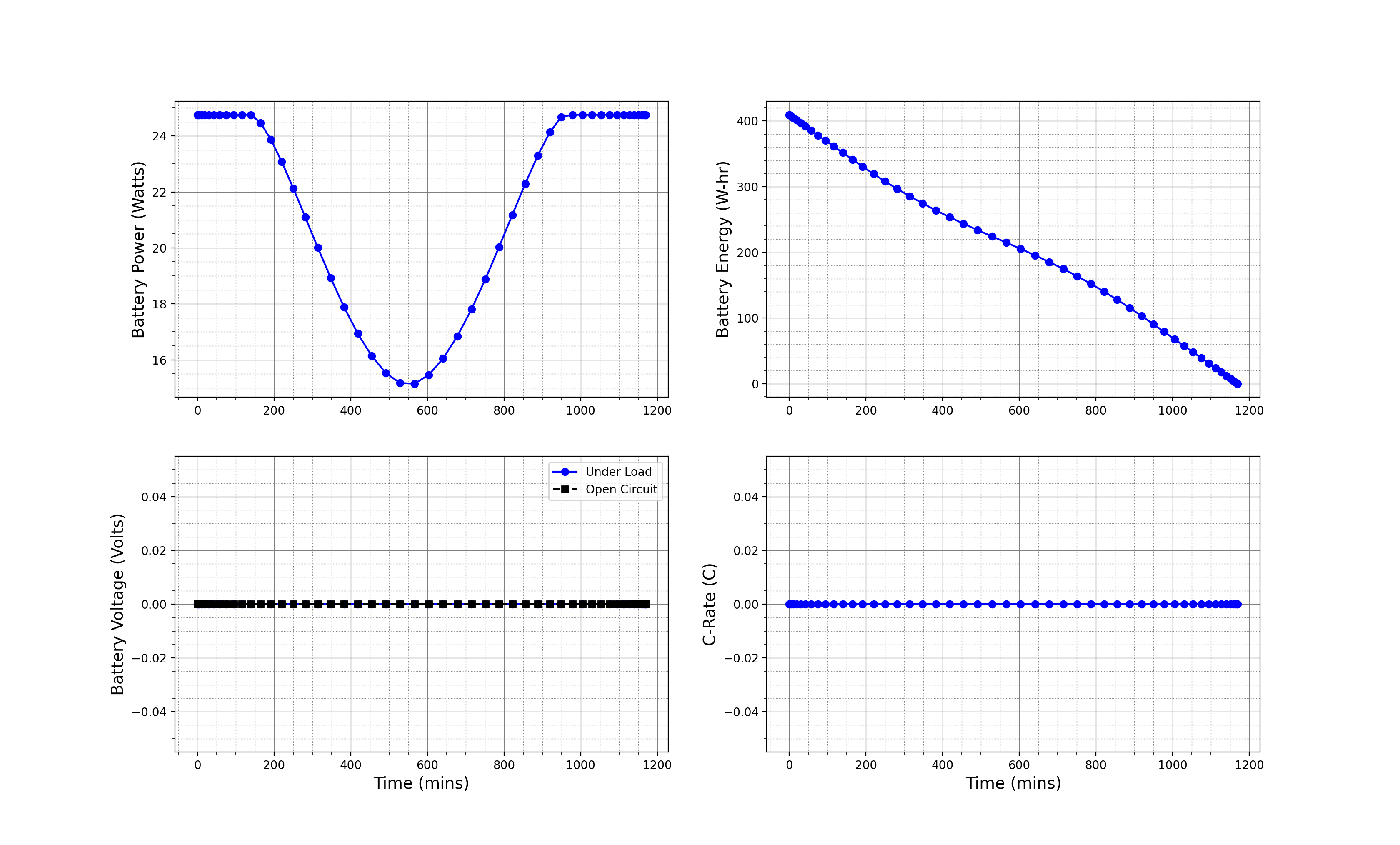
So we can tell now that the battery energy doesn’t go all the way to zero. One thing to note, because we have a solar UAV the voltage is regulated differently and the C-rate doesn't apply in the same way. Let’s look at how the solar flux varies throughout the day and how that affects the draw from the battery.
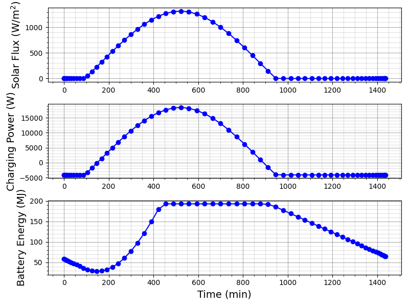
So maybe those solar panels actually are worth it. They seem to decrease the load on the battery considerably during the daytime.