Regional Jet Optimization Tutorial
This tutorial assumes familiarity with SUAVE and knowledge of the information in the Boeing 737-800 analysis tutorial. It provides a specific case of the more general optimization capabilities in SUAVE, and provides more information on how to modify the code for different uses.
Some important files for the optimization problem can be seen below
Important Files :
Optimize.py:
Defines the optimization framework of the problem, wherein one minimizes an assigned objective, subject to certain constraints, by altering some design variables.
In order to ensure that the subfunctions can communicate with eachother, and that SUAVE can communicate with the external optimizer, a special data object called the “Nexus” is used. The nexus object contains all of the vehicles, missions, results, and other important information. It alters these values at each optimizer iteration, depending on the input parameters defined in Optimize.py.
In this particular setup, there are two design variables: wing area and cruise altitude. The objective is to minimize fuel burn, and there is only one constraint: fuel margin. The default inputs are defined in the following lines.
    #   [ tag                   , initial,     (lb , ub)        , scaling , units ]
    problem.inputs = np.array([
	[ 'wing_area'           ,  80    , (   50. ,   130.   ) ,   100.  , Units.meter**2],
	[ 'cruise_altitude'     ,   8    , (    6. ,    12.   ) ,   10.   , Units.km],
    ])
Each input parameter takes in 5 values; a tag (an identification to communicate between the optimizer and SUAVE), an initial value, set of bounds, a scale factor (many optimizers tend to be more effective when the input values are of order 1), as well as the units used.
The objective and constraints are defined in the lines below.
	# [ tag, scaling, units ]
	problem.objective = np.array([
		[ 'fuel_burn', 10000, Units.kg ]
	])

	# [ tag, sense, edge, scaling, units ]
	problem.constraints = np.array([
		[ 'design_range_fuel_margin' , '>', 0., 1E-1, Units.less],
	])
Note that in this case, only a single constraint is used. Multiple constraints may be used using a list format, similar to the input variables.
This file also defines the “aliasing,” i.e. how the design variables, constraints, and objective map to the variables used in Procedure.py (which is where the problem is evaluated). The aliases for this problem are defined in the lines below. Note that the first entry refers to the tag defined in either problem.inputs, problem.objective, or problem.constraints.
	problem.aliases = [
		[ 'wing_area'                        ,   ['vehicle_configurations.*.wings.main_wing.areas.reference',
							  'vehicle_configurations.*.reference_area'                    ]],
		[ 'cruise_altitude'                  ,    'missions.base.segments.climb_5.altitude_end'                 ],
		[ 'fuel_burn'                        ,    'summary.base_mission_fuelburn'                               ],
		[ 'design_range_fuel_margin'         ,    'summary.max_zero_fuel_margin'                                ],
	]
Note that, sometimes, a single input can map to multiple outputs, such as the “wing_area” design variable; in this case, use a list for the outputs, as seen above. The use of a wild card “*”, can also allow values to map to multiple outputs. Values to be outputted cannot contain wild cards as that would be ambiguous to an optimizer.
Procedure.py:
This links everything together by defining the steps you would use to size and analyze the aircraft at each optimizer iteration.
This file contains a number of subfunctions to alter the vehicle and mission. The function setup() instantiates the procedure, defining the functions that are called at each step of the optimizer in their order of execution.
-
simple_sizing() defines the geometry of the aircraft based on the input parameters (in this case, wing area and cruise altitude).
-
weights() determines the weight breakdown of the aircraft
-
mission() decides which missions are run at each step, as well as the design mission of the aircraft
-
post_process() handles the results from the missions, saving the constraints and objective value
Each step of the procedure takes the nexus object as an input, and returns the object as an output, ensuring that the data is available for handling.
Vehicles.py:
Initializes the vehicle (or vehicles if desired) used in the optimization problem. This includes two subfunctions: base_setup(), where the vehicle structure is itself defined, including the fuselage, wing, vertical and horizontal tails, and the propulsion system.
configs_setup() takes in the vehicle that was defined in base_setup() and defines other configurations (such as takeoff and landing, which include different flap settings). This may be used to define other parameters, such as changing the sweep angle of a variable-sweep-wing at higher Mach Numbers, or changing a propulsion component.
Missions.py:
Initializes the missions that are run at each iteration. In this case, only a single mission is run.
Analyses.py:
Defines the set of features that are used in this particular problem (e.g. weights correlations, aerodynamics correlations, etc.).
Plot_Mission.py:
Plots the mission outputs.
Running the Problem:
-
Locate the tutorial script folder “Regional_Jet_Optimization.”
-
Open the Optimize.py script in a text editor or IDE. You will see this line near the top of main():
output = problem.objective() -
This runs the problem with the default inputs. Run the file using an IDE or type
python Optimize.pyin the command line. You should see a set of output plots.
Running a Sweep of the Inputs
Now try running a 2D sweep of the problem to observe the shape of the design space: comment output = problem.objective then uncomment the following (the next line down in the code).
variable_sweep(problem)
Then run the program again. This could take a few minutes. The results should look like the plot below.
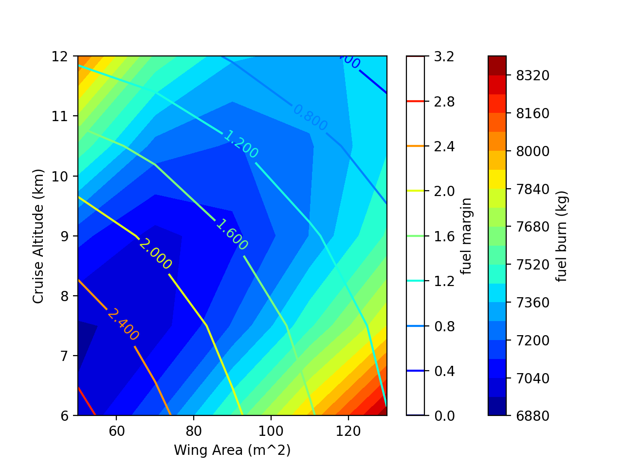
The labeled lines depict the fuel margin (i.e. fraction of the aircraft remaining weight that can be loaded with fuel). Positive values indicate a feasible design. Fuel burn is shown in the colored contours. Note that a smoother plot may be created by changing the number of points in the sweep function, but this will take more time. A carpet plot run using 400 points on can be seen below. A local minimum is now visible.
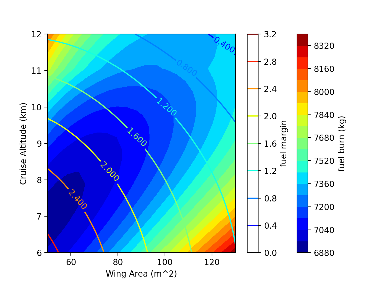
Note: If you run this 400 point case yourself you may see messages indicating that a segment did not converge. This is normal and can happen when a mission is run far from a feasible point. In this case, it does not have a negative impact on the results.
Optimizing:
Now try running an Optimization. Recomment variable_sweep(problem) then uncomment the lines below:
	output = scipy_setup.SciPy_Solve(problem,solver='SLSQP')
	print output
and run the file again.
From the default inputs, the terminal (or IDE output) should display an optimum of [0.57213139 0.75471681] which corresponds to a wing area of 58 m^2, and 7.5 km. It appears to have found a minima. Keep in mind that in designing a real regional jet the desingers would incorporate additional constraints and analyses. These additional constraints change the final design considerably
At this point, you can explore other starting points, or alter the vehicle or mission properties in Vehicles.py or Missions.py. Additionally, feel free to start using this as the basis for creating custom optimization scripts.