Introduction
The purpose of this tutorial is to educate users on how to setup a preconfigured solar energy network to work with a high altitude solar UAV. In this tutorial it is assumed that the user has some familiarity with SUAVE having completed the fundamental tutorial for the Boeing 737-800. You will learn about setting up the following:
- Solar missions,
- Human powered/solar weight estimation,
- Boundary layer transition,
- Solar panels,
- Batteries,
- Electric motors,
- Propellers,
- Electric network integration in a solar UAV
Because of the flexible nature of SUAVE, the approach shown is just one way to setup the UAV for analysis. By experimenting and eventually developing your own code you will be able to do far more than what is shown in this tutorial. The original script can be found in the tutorial repository as tut_solar_uav.py.
Vehicle and Mission
The vehicle is similar to the Qinetiq Zephyr but far larger at 40 meters in wing span and a weight of 200 kg. However, it does carry double the payload of the Zephyr at 5 kg and accounts for constant payload power usage. The battery energy density is set to an optimistic estimate of 450 Watt-hours per kg. Additionally, 90 percent of the wings are covered with solar panels that have a 25 percent efficiency.
This mission exercises the methods developed for solar radiation estimation, propeller and motor integration, as well as the human powered aircraft weight estimation. The mission setup is a constant altitude cruise at 15 km at Mach 0.12 for about 24 hours. The location is over the California Bay Area during the summer solstice.
Setup
This tutorial highlights the differences between setting up a typical commercial aircraft like a Boeing 737 and a solar UAV.
Mission Setup
For a solar UAV, the starting location as well as the day and time are critical. So the first segment must be modified to include this information. It is important to note that the start times provided are in “Zulu” time or Greenwich Mean Time. This is typical for aircraft navigation to prevent time zone errors and ambiguity.
segment.state.numerics.number_control_points = 64
segment.start_time                           = time.strptime("Tue, Jun 21 11:30:00  2020", "%a, %b %d %H:%M:%S %Y",)
segment.altitude                             = 15.0  * Units.km
segment.mach                                 = 0.12
segment.distance                             = 3050.0 * Units.km
segment.battery_energy                       = vehicle.propulsors.solar.battery.max_energy*0.2 #Charge the battery to start
segment.latitude                             = 37.4300   # this defaults to degrees (do not use Units.degrees)
segment.longitude                            = -122.1700 # this defaults to degrees
Additionally, this mission is highly simplified. It consists of only one mission segment. To provide ample resolution, the number of control points has been increased to 64.
Structural Weight Sizing
The vehicle sizing of the human powered aircraft or solar UAV requires the dimensions of the vehicle like in other weight estimation methods. However, it also requires information about the number of wing ribs and the number of end ribs. The end ribs are relevant for wing designs where the sections can come apart for transportation.
wing.number_ribs             = 26.
wing.number_end_ribs         = 2.
Wing Boundary Layer Transition
The transition location of the boundary layer can have a great impact on the drag of the wing. This is especially important in properly designed, low Reynolds number flows, where laminar flow can be extended for larger regions of the surface. The code snippet below is how surfaces have transition points set. These are estimates provided from the designer based on experience.
wing.transition_x_upper      = 0.6
wing.transition_x_lower      = 1.0
Solar Panels
The solar panel model is quite simple and only requires a capture area, an efficiency, and mass. In this case we assume that 90% of the wing area is covered in solar panels.
panel.area                 = vehicle.reference_area * 0.9
panel.efficiency           = 0.25
panel.mass_properties.mass = panel.area*(0.60 * Units.kg)
Batteries
The batteries are set up with knowledge of the mass of the battery and the specific energy. In this case a futuristic specific energy of 600 Watt-hr/kg is set for lithium ion type batteries. The resistance of the batteries is another important input to determine charging and discharging losses.
bat = SUAVE.Components.Energy.Storages.Batteries.Constant_Mass.Lithium_Ion()
bat.mass_properties.mass = 90.0 * Units.kg
bat.specific_energy      = 800. * Units.Wh/Units.kg
bat.resistance           = 0.05
bat.max_voltage          = 45.0
initialize_from_mass(bat,bat.mass_properties.mass)
net.battery              = bat
Propeller
To setup the propeller we will actually design an optimized propeller. This is done through the methods provided by Adkins and Liebeck. The attributes of the propeller design are then seeded to the motor and network to accelerate convergence of the propeller and motor models.
prop = SUAVE.Components.Energy.Converters.Propeller()
prop.number_blades       = 2.0
prop.freestream_velocity = 40.0 * Units['m/s']# freestream
prop.angular_velocity    = 150. * Units['rpm']
prop.tip_radius          = 4.25 * Units.meters
prop.hub_radius          = 0.05 * Units.meters
prop.design_Cl           = 0.7
prop.design_altitude     = 14.0 * Units.km
prop.design_thrust       = None
prop.design_power        = 3500.0 * Units.watts
prop                     = propeller_design(prop)

net.propeller            = prop
Motor
This motor model relies on data that is generally available from motor manufacturers. This includes the resistance, no load current, and the speed constant. Additionally, any gearbox is specified here and basic information about the propeller is entered here to help inform the solver when converging the motor and propeller analyses.
motor = SUAVE.Components.Energy.Converters.Motor()
motor.resistance           = 0.008
motor.no_load_current      = 4.5  * Units.ampere
motor.speed_constant       = 120. * Units['rpm'] # RPM/volt converted to (rad/s)/volt
motor.propeller_radius     = prop.tip_radius
motor.propeller_Cp         = prop.power_coefficient
motor.gear_ratio           = 12. # Gear ratio
motor.gearbox_efficiency   = .98 # Gear box efficiency
motor.expected_current     = 160. # Expected current
motor.mass_properties.mass = 2.0  * Units.kg
net.motor                  = motor
Running
As you should be familiar with by now, running this script is just like any other.
python tut_solar_uav.py
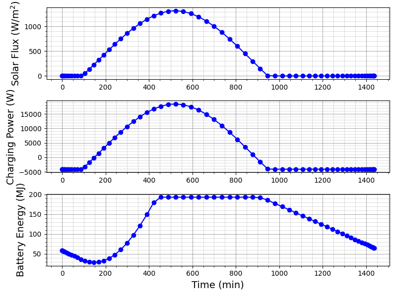
Results
If all went well the script ran and it provided you with more plots than you ever wanted. Here are some of the plots that were generated when we ran it: